Tshark Examples – Theory & Implementation

This blog is a merger of two past blogs we did revolving around T-shark. The first blog explains how to extract fields (aka the theory) and the second blog shows you one of the many things you can do with that feature (aka the implementation).

 

Theory

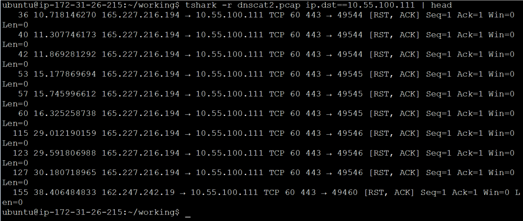
In a previous blog entry, I referenced using tshark to extract IP header information so that it could be sorted and analyzed. I had a number of questions around how this works, so I wanted to post a more in-depth blog entry that discusses tshark’s ability to display specific header fields. I’ll also dive into how these fields can be extracted and manipulated. For reference, here’s the screen capture that started the conversation:

Let’s break down some of the components of this command.

 

Reading Capture files With Tshark

By default, tshark will listen on the local interface in order to grab packets off the wire. If you have a pcap file that you wish to process, you can use the “-r” command. If you will be printing the output to the screen, I like to pipe the output through “head” (show only a specified number of lines of output) or “less” (show one full page of output at a time) so that it’s easier to read. For example:

tshark -r interesting-packets.pcap | head

By default “head” will show the first 10 lines of output but you can modify this as needed, feeding it the number of lines you want to see as a command-line switch. For example in the first screen capture, I used “head -20” to print the first 20 lines of output.

 

Filtering Traffic With Tshark Capture Filters

When we review a pcap file, there is usually a specific characteristic we are looking for. For example, we may wish to examine all traffic associated with a specific IP address or service. Capture filters permit us to start honing in on an interesting pattern.

If you are a Wireshark user, capture filters work a bit differently with tshark versus Wireshark. Tshark actually uses the Wireshark Display Filter syntax for both capture and display. This is pretty cool as it provides a lot more functionality. The syntax for tshark capture filters is:

<field><operator><value>

Some examples would be:

ip.dst==192.168.1.10 
ip.proto==17 
tcp.flags.reset!=0

Note that in the second example I have to use the protocol number (17) instead of the protocol name (UDP). This is pretty common for most filters. Use the Wireshark Display Filter syntax page I referenced above to identify the proper format to use. In the first two examples, I use the operator “==” to identify that the value must be a match. Note that in the last example I use “!=” which means not equal to. You can also use greater than ( >> ), less than ( << ), equal to or greater than ( >= ) or less than or equal to ( <=).

Also, note that in the last example I’m matching on a single bit (reset bit in byte 13 of the TCP header). This means I need to identify if I’m interested in the bit being on (represented by a “1”) or off (represented by a “0”). So another possible way to write that last example would be:

tcp.flags.reset==1

If I’m interested in traffic associated with a specific IP address, I could build on the “-r” command above as followed:

tshark -r interesting-packets.pcap ip.dst==192.168.1.10 | head

 

Redirecting Tshark Output to a New File

Sometimes it is helpful to read an existing pcap file and redirect the output to a new file. For example, what if I wanted to take all traffic associated with a specific IP address and put that in a different file for further analysis? This would permit me to review this new file and possibly refine my filtering even further. We can use “-w” to create a new capture file. Here’s an example:

tshark -r interesting-packets.pcap -w interesting-host.pcap ip.dst==192.168.1.10 | head

 

Selecting Which Fields to Output With Tshark

By default, tshark will print a brief summary of each packet which includes various header fields. Here’s an example:

While this is handy when performing a quick decode, what if the information we wish to review is not in the default output? What if we only want to see one or two of the fields but not everything else? Luckily tshark lets us specify the exact fields we wish to see.

We can use the command line switch “-T fields” to identify that we wish to specify the exact fields to print rather than showing the default information. We can then use “-e” to identify which specific fields to print. The values I use with “-e” are the Wireshark Display Filters I mentioned earlier. Here’s an example that would print just the source and destination IP address:

tshark -r interesting-host.pcap -T fields -e ip.src -e ip.dst ip.dst==192.168.1.10 | head

This would produce output similar to the following:

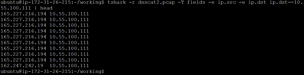
If I want to organize this for viewing, I can add the “-E header=y” switch as shown in the first screen cap. This will print out the first line of column titles. While this can be helpful if you will be importing the data into a spreadsheet, I don’t recommend it if you will be manipulating data from the command line. This is because the column titles may get mixed in with the data.

 

Organizing Tshark Fields For Additional Processing

Let’s assume we want to extract certain fields out of our packets and move them to a file for further processing. The first thing we should do is print the interesting fields but use a consistent column separator so that the values will be easier to pass to other tools. For this, we will use the “separator” switch and set it to use a comma. Here’s an example command:

tshark -r interesting-host.pcap -T fields -E separator=, -e 
ip.src -e ip.dst ip.dst==192.168.1.10 | head

This will give me output similar to the last example, but with commas instead of spaces between the printed values. Finally, rather than printing to the screen, we should redirect the output to a text file. This way we can feed that file into additional tools for processing. Here’s an example:

tshark -r interesting-host.pcap -T fields -E separator=, -e 
ip.src -e ip.dst ip.dst==192.168.1.10 > analyze.txt

This will result in a text file where each line contains information extracted from a single packet. The line will include the source and destination IP address separated by a comma.

 

Manipulating Tshark Output

Which tools I should use to manipulate the data depends on the goal I’m trying to achieve. Linux has a wide range of text manipulation tools such as cut, sort, uniq and grep. With a bit of Google searching, you can find a ton of useful write-ups on using each of these tools. For this blog entry, I want to cover the “R” command as it permits us to do some statistical analysis.

Here’s the command I used to generate data output similar to the first screen capture, but in a format, I can use for beacon analysis:

tshark -r interesting.pcap -T fields -E separator=, -e 
ip.src -e ip.dst -e ip.proto -e udp.dstport -e ip.len -e 
frame.time_delta_displayed ip.dst==165.227.88.15 and udp.dstport==53  > analyze.txt

This produced a file called “analyze.txt” which contained data similar to the following:

192.168.88.2,165.227.88.15,17,53,89,1.073288580 
192.168.88.2,165.227.88.15,17,53,89,1.067193833 
192.168.88.2,165.227.88.15,17,53,89,1.057524219 
192.168.88.2,165.227.88.15,17,53,89,1.085981806 
192.168.88.2,165.227.88.15,17,53,89,1.072384382

It is the last two fields I’m interested in analyzing. With beacon analysis, I want to look for repeating patterns. Consistency in both session data size and timing can be indications of an internal system that has been compromised and is calling home. One way to check for repeating patterns is to analyze the standard deviation and the variance of the data. Luckily the R command can do this for us.

I’m going to use “cut” to extract the column of data that I’m interested in analyzing, and then use R to identify the minimum, maximum, mean, standard deviation, and variance of the data set. Here’s an example:

cut -d ',' -f 5 analyze.txt | Rscript -e 'y <-scan("stdin", quiet=TRUE)' 
-e 'cat(min(y), max(y), mean(y), sd(y), var(y), sep="\n")' 
89 
290 
95.74 
33.82236 
1143.952

In the above example, “cut” extracts column 5 which is the amount of data transferred in each session. It then passes these values to “R” which calculates the minimum, maximum, mean, standard deviation and variance for this data set. Note that my standard deviation is much larger than the difference between the mean and the minimum value. This tells me that most of my sessions are closer to the minimum 89 byte size. This is somewhat interesting because it indicates that the majority of traffic exchanged between these two systems involved sessions with a small amount of data. This could be indicative of a beaconing heartbeat but is certainly not conclusive.

I can perform a similar analysis on the session timing:

cut -d ',' -f 6 analyze.txt | Rscript -e 'y <-scan("stdin", quiet=TRUE)' 
-e 'cat(min(y), max(y), mean(y), sd(y), var(y), sep="\n")' 
0 
2.088164 
0.9999386 
0.2973222 
0.08840052

This is where things get really interesting. Note that the maximum gap between sessions is just a bit over two seconds. This is extremely frequent. Also, note that the variance from the mean is just .08840052 seconds or about 88 ms. This tells us that an overwhelming majority of the communication sessions are taking place almost exactly .9999 seconds apart from each other. This is a clear indicator of a beacon heartbeat.  Based on this data, if I did not expect to see beacon behavior between these two systems, I would want to subject the internal system to a forensic analysis.

 

Summary

One of the challenges of packet analysis is honing in on the interesting bits and ignoring everything else. This can be a challenge with the default view in most packet decoders, as you either get too much information or not enough. Further, while graphical analysis tools can be easy to use, they make it difficult to leverage other tools or automate an analysis. By leveraging tshark’s ability to print specific fields, you can manipulate data as needed to perform an in-depth analysis.

 

Implementation

 

Video – Catching Data Exfiltration With a Single Tshark Command

 

 

 

 

 

Command Used

tshark -r data-exfil.pcap -T fields -e ip.src -e ip.dst -e ip.len ip.src == 192.168.0.0/16 or ip.src == 10.0.0.0/8 or ip.src

 

Video Transcript

(00:00)
Hey folks, I’m Chris Brenton and today I’m going to show you how to identify which of your internal systems are sending the largest amount of data out to the internet using a single TShark command.

(00:12)
Now, first, a couple of caveats. Number one, this does not work as a live capture, meaning I can’t sniff the traffic off the network live in order to get this information, I need to read it out of a capture file. The longer the capture file, the better. Preferences like 24 hours collected off of the internal interface of the firewall. That way you’re seeing all the internal systems as they go out to the internet.

(00:34)
Another caveat here, this is slow. I did another video on how to do exactly the same thing as Zeek. If you’re going to be doing this on a regular basis, I highly recommend you use Zeek instead, but if you’ve got a pcap file and you’re in a pinch, here’s an easy way to go through and do that.

(00:51)
The third caveat I have is that the amount of data that I’m going to display as being sent out is not 100% accurate. It’s also going to include the IP header in each packet, which is 20 bytes. So we’re going to see a little bit more data transfer it out than what was actually in the payloads. But when you start looking at comparing it to other systems, it’s still apples to apples.

(01:18)
So those are the caveats. With that said, here’s what we’re doing. We’re using TShark’s ability to go in and extract out certain fields. We’re pulling out the source IP, the destination IP, and the size of the IP packets. We’re then going in and creating a filter that says, “Only show me the data that was transmitted by my systems on the internal network.”

(01:38)
We’re sorting the data, we’re running it through Datamash. Datamash is going to go through and add up multiple sessions between the same two IP addresses and give us a sum total so we can see the total number of bytes. And then we’re just sorting it out from highest to lowest. Looking at our top 10, and the result is what we get here. Now I’m noticing a couple of patterns. I’m noticing that 10.55.100.111 seems to be sending the most amount of data out to a bunch of different IP addresses out on the internet. So where should I begin my investigation? That would be the system I’d go after first. That’s it. Hope you found this video useful.